Solve any optimization problem using Julia

JuliaLang Community has created different packages to solve optimization problems. For instance, Metaheuristics.jl implements high performance metaheuristics for solving global optimization problems.

 

Installing Metaheuristics

 

Open the Julia (Julia 1.1 or later) REPL and press ] to open the Pkg prompt. To add this package, use the add command:

pkg> add Metaheuristics

Or, equivalently, via the Pkg API:

julia> import Pkg; Pkg.add("Metaheuristics")

Algorithms

Some representative metaheuristics are developed here, including those for single- and multi-objective optimization. Moreover, some constraint handling techniques have been considered in most of the implemented algorithms.

Single-Objective Optimization: Those problems consider only one objective function and may or not consider constraints.

• ECA: Evolutionary Centers Algorithm

• DE: Differential Evolution

• PSO: Particle Swarm Optimization

• ABC: Artificial Bee Colony

• GSA: Gravitational Search Algorithm

• SA: Simulated Annealing

• WOA: Whale Optimization Algorithm

Multi-Objective Optimization: Those problems have two or more conflicting objective functions to be minimized simultaneously.

• MOEA/D-DE: Multi-objective Evolutionary Algorithm based on Decomposition

• NSGA-II: A fast and elitist multi-objective genetic algorithm: NSGA-II

• NSGA-III: Evolutionary Many-Objective Optimization Algorithm Using Reference-Point-Based Nondominated Sorting Approach

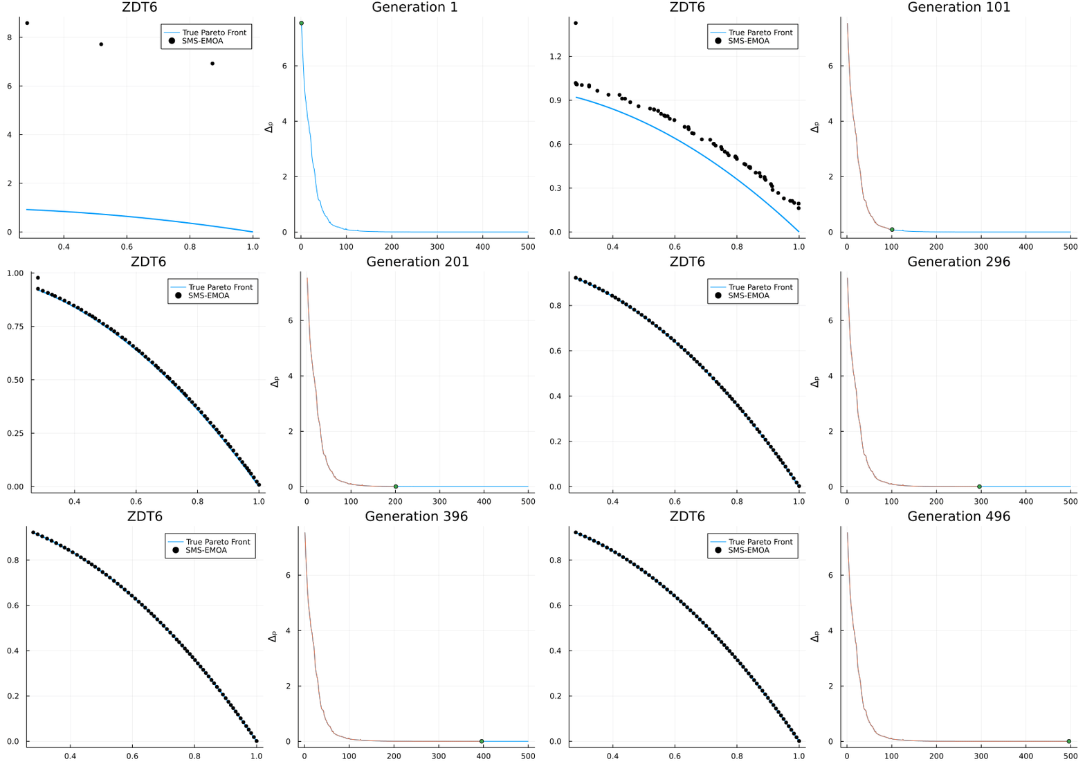
• SMS-EMOA: An EMO algorithm using the hypervolume measure as selection criterion

• SPEA2: Improved Strength Pareto Evolutionary Algorithm

Performance Indicators 

Performance indicators are used to compare the algorithms performance in order assess the results given by one or more methods for optimization.

• GD: Generational Distance

• IGD, IGD+: Inverted Generational Distance (Plus)

• C-metric: Covering Indicator

• HV: Hypervolume

• Δₚ (Delta p): Averaged Hausdorff distance

• Spacing Indicator

• and more…

Example

This example illustrates how implement and solve an optimization problems by sing Metaheuristics.

Firstly, import the Metaheuristics package:

using Metaheuristics

Code the objective function:

f(x) = 10length(x) + sum( x.^2 - 10cos.(2π*x)  )

Instantiate the bounds, note that bounds should be a Matrix where the first row corresponds to the lower bounds whilst the second row corresponds to the upper bounds.

D = 10
bounds = [-5ones(D) 5ones(D)]'

Approximate the optimum using the function optimize.

result = optimize(f, bounds)

Optimize returns a State datatype which contains some information about the approximation. For instance, you may use mainly two functions to obtain such approximation.

@show minimum(result)
@show minimizer(result)

Documentation

See the documentation for more details, examples and options.